[0:10]Hello and welcome to lecture 24 of Analog Integrated Circuit Design. In this lecture, we will deal with one of the very important non-ideal features of any real circuit, that is random noise. It turns out that dissipative components like a resistor or a MOSFET have random noise, and components which don't have any power loss like capacitors and inductors don't. So we, in this lecture, we'll look at the random noise on a resistor.
[0:49]As Ohm's law says, if you pass a current I through a resistor R, the voltage across that should be I times R. And if you apply a voltage source V across a resistance R, the current through that will of course be V divided by R. Now in reality, because of random motion of carriers through the resistor, the current is not exactly V by R. Okay? Let's say you take this circuit and measure the value of I very, very precisely versus time. You will see that the current has a mean value of V by R, but there are variations around this mean value. And that happens because if you take any cross-section of a resistor, let's say a current I is flowing that way, I equals V by R. That means that on average, this much charge is flowing every second through the resistor. But if you do take a cross-section, and see the charge flowing across the cross-section, in addition to this average value, there will be charges randomly moving back and forth across the cross-section. This is because of random thermal motion of charges. Okay? As long as the temperature is above absolute zero, this is going to happen. Now we need a way to quantify this and also to estimate it in any given circuit. Okay? Clearly, because of this, the current in any circuit is not exactly what we calculate based on the device relationships. Okay? First of all, the resistor noise, it turns out that if you do this experiment with two different resistors,
[3:10]the noise waveform that you see here will not be the same. They'll be uncorrelated from one resistor to another. Okay? It's a random phenomenon and what's happening in one resistor doesn't have anything to do with what happens in another resistor. It also, it turns out that in the particular case of a resistor, it is uncorrelated from one time instant to another.
[3:50]Okay? So if you take the value at a particular time and another time in the same resistor, they will also be uncorrelated from each other. Okay? How can we quantify something that is random such as this? There are many ways. From your study of probability and random processes, you will know that you can specify the power spectral density or in general, the spectral density which relates to how the randomness, the energy in the randomness is distributed over frequency. Okay? You can also specify the mean squared or the root mean squared value, one of these things.
[4:47]And for zero mean random processes, these are the same as the variance and the standard deviation. Okay?
[5:01]Now in this case, we assume that the average current is V by R and the rest of it is noise, and by definition, it will have zero mean. Okay? So we can either call it the root mean squared value or standard deviation or either mean squared value or variance. Okay? We have to specify one of these things to specify the size of the noise. Because noise is random, we can't specify the amplitude. In fact, theoretically, the amplitude of such a noise, it turns out to be infinity. But we can specify the size of the noise by specifying the mean squared value of the noise. Okay? We need to learn how to do this for a resistor. First of all,
[5:38]let me go back to the two pictures I drew earlier. If I have a voltage source across a resistance, the current I equals V by R plus some noise current. Okay? And this can be modeled by assuming that there is a noiseless resistor and a noise current source across it.
[6:14]Okay? The arrow is just to symbolize that it's a current source. It doesn't mean that the current is always in this direction. As I said, the mean value of I is zero, and the current can flow in both directions. Clearly in this case also, I will be equal to V by R due to the noiseless resistor plus I N. Okay? So we model the noise in the resistor as a current source. Okay?
[6:45]If I look at the alternative description, if I pass a current I through a resistance R, the voltage across it will be I times R plus a noise voltage. And this again can be thought of as the current flowing through a noiseless resistor and a series voltage source, which is equal to the noise voltage. Okay? In this case also, the voltage across it is I times R plus V N.
[7:22]So in the pictures on the right side, what is done is the noise itself is abstracted out as a source. And this is a very common thing. You assume that there is a noiseless component which follows the VI relationships that you know. It is Ohm's law for a resistor or square law for a MOSFET and so on. And the noisy part of it is modeled out as either a voltage source or a current source, whichever is convenient. Okay? Now, finally, if we are going to use this model or that model for a resistor, the two have to describe the same thing. Okay? And that will happen if I N times R equals V N. Okay? This we can see very easily by assuming that let's say we have applied a zero voltage source across the resistor.
[8:47]And I short circuited, just like here. Clearly, the current here will be V N divided by R. Okay? And the currents here and here have to be the same, so that means that the equivalent voltage source of a resistor and equivalent current source of a resistor are related by a ratio, which is equal to the resistance R. Okay? As I mentioned before, we cannot specify the instantaneous value of either I N or V N. Okay? So what we will specify instead is the spectral density, that is, how the energy in V N or I N is distributed over frequencies. Okay?
[9:53]Now, first of all, what is the spectral density? Spectral density is some function of frequency. And as is common in circuit design, we take the one-sided spectral density. That means that we specify the spectral density for positive frequencies. And what the spectral density tells you is some function. The spectral density of I N will be some S I of F. Okay? And what is this? This is related to the Fourier transform of the auto-correlation function.
[10:46]And in particular, the integral of S I over all frequencies, zero to infinity will be equal to the auto-correlation function at a time shift of zero, or the variance, sigma squared. So this is how the spectral density is useful in specifying the magnitude of the noise. Okay? Now for a description of auto-correlation function, spectral density and so on, you can refer to any basic book on random processes. It turns out that in the particular case of a resistor, if I plot the spectral density of the current, it is constant for all frequencies. Okay? And such a function is known as white noise. Okay? If the spectral density of a certain noise process is constant for all frequencies, it's known as white noise, analogous to white color, which has all frequencies in it. Okay? And the magnitude of that spectral density is 4 K T divided by R, where K is Boltzmann's constant, 1.38 times 10 to the minus 23 joule per Kelvin.
[12:24]Okay? And T is the absolute temperature. Room temperature corresponds to 300 Kelvin. Okay?
[12:49]Now, we also know that the noise voltage is related to the noise current by a multiplicative factor R. So the noise spectral density of the voltage is related to the noise spectral density of the current by the square of the multiplying factor. Okay? This is because basically the spectral density relates to the square of these quantities. Okay? So that means that the noise voltage of a resistor has a spectral density, which is 4 K T divided by R, times R squared, equals 4 K T R. Okay?
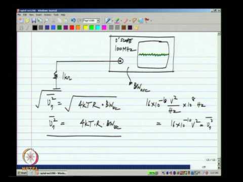
[13:34]Naturally, that is also constant with frequency and it is 4 K T R. Good numbers to remember are that K T equals 4 times 10 to the minus 21 joules at 300 Kelvin. Okay? And if you calculate let's say for R equals 1 kilo ohms, what we will get is 4 times 4 times 10 to the minus 21 joules times 10 to the 3 ohms, and this gives to 16 times 10 to the minus 18 volt squared per Hertz. Okay?
[14:22]The voltage noise is specified in volt square per Hertz. It is related to the square of the voltages, and the spectral density obviously relates to a density over frequency. So it is given in volt square divided by Hertz, or volt square per Hertz. Okay? Similarly, the current noise spectral density is given by units of ampere square per Hertz. Okay?
[14:48]So S I is 4 K T divided by R ampere square per Hertz, and S V is 4 K T R volt square per Hertz. Okay? And as I mentioned, for a 1 kilo ohm resistor, S V turns out to be 16 times 10 to the minus 18 volt square per Hertz. And clearly from that we can also calculate S I, which is 16 times 10 to the minus 24 ampere square per Hertz. Okay? Now we didn't derive any of these results. We just took them for granted. These results were derived by Nyquist long long ago, and they have been used very widely and then confirmed experimentally and so on. Okay? But what does it mean? I mean, we have these abstract descriptions of noise in terms of the spectral density and so on. And we said something about it being related to distribution of these quantities over frequencies. But when we deal with circuits, we deal with voltages and currents. Right? I have a 1 volt signal here and I have a 10 mV signal there and so on. Now noise is something that is random, and I should like to specify it also in terms of voltages or currents. Okay? Then I can compare my signal to the noise and see if the signal is sufficiently above noise. Now from common experience, you know that if you are trying to decode some signal or let's say you're trying to listen to something, and there is a lot of noise, you will not be able to if there is very little noise, you can. Okay? So you have to be able to quantify the amount of signal to the amount of noise. And for that, we need to be able to describe the signal and noise in the same units, and we describe the signals in terms of voltages or currents. Similarly, we have to do the same for the noise as well. Okay?
[16:45]So what is the meaning of the spectral density then? What it means is that let's take some values. Let me take C to be 10 pF.
[19:00]Let me take R to be, let's say, 100 k ohms. So 1 over 2 pi C R equals 1 over 2 pi times 10 to the minus 11 times 10 to the 5 equals 10 to the 6 by 2 pi Hertz. Okay?
[46:21]So let's say it is somewhere here, and then it drops down to 8 and then drops off like that. Okay? And what is the variance after all? It is the area under the spectral density curve from zero to infinity. Okay?
[50:37]So what does this mean? The variance of this will be infinite because the bandwidth is infinite. Right? 4 k t r integrated from zero to infinity will be infinite. So if I take a resistor and measure the voltage across it, will I measure infinity? What do you think? When clearly not, because if you do have infinite voltage across the resistor, none of the small signal assumptions would be true and no circuit that you make will you will ever work. So many things happen. First of all, your measuring instrument will have some finite bandwidth. So that will limit the amount of voltage that it measures. Okay? So that is one thing. And a resistor itself will have some parasitic capacitance across it, because between any two terminals there'll be some capacitance. And across every resistor, there will be some capacitance, however small. If you make the resistor physically smaller, the capacitance will be smaller and so on. Okay? So that is another thing that limits the noise. But even more fundamentally, the noise itself turns out to be not white. Okay? This again I will not elaborate on, but from your first year physics courses you may remember what is known as the ultraviolet catastrophe that led to the introduction of quantization and quantum mechanics. Okay? So initially, it was assumed that the distribution of energy across frequencies was uniform. And then it led to this prediction that a black body will radiate infinite power. And that was resolved by Max Planck, who postulated that the energy is only in discrete packets, and that is proportional to the frequency of the radiation.
[52:11]And that gives you a result that makes sense, that it has a finite energy. Okay? And the result of all that is that basically, this KT will be replaced by H new divided by exponential H new by KT minus 1. Okay? So this KT is something independent of frequency, but this function is very much dependent on the frequency. And H is Planck's constant and new is the frequency. And you can very easily also see that when the frequencies are very small, H new is much smaller than KT, this reduces to KT. Okay? So essentially, what we have is a low-frequency approximation to the reality. H new by exponential H new by KT minus 1 approximates KT for very low frequencies. And that low frequencies includes frequencies up to terahertz and so on. So we can safely use this white assumption for all our circuits. Okay? Thank you. In the next lecture, we will deal with the noise in other components like the MOSFET.


