[0:00]name is Dr. Storm Kennedy Palmer. I'm the secondary lecturer for this module. Um and today we are going to be looking at learning unit nine. I assume you did the previous week's session to to look at part A of this, but I'm going to do a quick revision for us as well. Please jump in whenever you have a question. You can either unmute yourself or um write it in the chat. I'll try to keep an eye open on the chat. But yeah, if if I don't if I don't see your comment please just unmute yourself and and ask it. So for this learning unit, um in the first session, you would have covered the first four learning unit outcomes, which were the relation between inflation, expected inflation and unemployment, the Phillips curve, the Phillips curve and the natural rates of unemployment and the ISLMPC model. Now, we're going to be looking at the adjustment from the short run to the medium run and the impact of fiscal policy using the ISLM-PC model. So remember then when adding the PC curve to the IS model, it adds the inflation dynamics showing how changes in output and unemployment affect the change in inflation over time. Together the ISLMPC curves explain how changes in fiscal policy, which would be government spending or taxation, and monetary policy, which would be repo rate changes, impact the economy's output and inflation in the short run. Thus in the short run, demand determines output. So in the short run, we can have a situation where output exceeds the natural level of output, which is illustrated in this diagram 9.3 from the learning unit. See that the equilibrium level of output Y is above Y in. Our current equilibrium level of output and income is above the natural level denoted by YN and the change in inflation is positive, meaning inflation is increasing. So this would be a zero change in inflation, okay, which doesn't mean that there's no inflation. If the change in inflation is zero, the inflation rate itself could be positive, like 6%, but it just when the change in inflation is zero, it means that the inflation rate is remaining at the previous period's inflation rate. So if it was 6% last period, it's 6% again this period because the change is zero. Now, this is positive. So imagine this is plus 2%, for example. That means that if in the previous period our inflation was 6%, we now add two and our inflation rate will be 8%. But as long as it stays as the change in inflation being positive, that will keep increasing. So as each period um passes, as we go through time, the change in inflation is positive, so the actual inflation rate keeps increasing period on period, year on year, whatever period we're dealing with in this particular example.
[5:00]And that means that the central bank because its target is to protect the value of the South African rand, that means not letting hyperinflation take over and degrade the value of the rand. So the central bank is going to come in and increase interest rates to combat this inflation that we're seeing here. So very important, I want you to remember, in the short run, output can be higher or lower than the natural level of output. We assume that actions taken by the Central Bank, however in the medium run, will mean that the level of output and income is equal to the natural level in the medium run. Now, I want to just go over this simple example to make sure there isn't any confusion between the concepts of constant inflation and rising or falling inflation. So, for the sake of simplicity, let's say we have a basket of goods in year one that costs 100 rand. What will the cost of this same basket be if inflation is 10%?
[6:14]It's easy. We just say a hundred and ten divided by 100. Okay, so you can see that it is a 10% increase, which gets us to 110 rand. So if our basket cost us 100 rand in year one, if there's a 10% increase in the following year, that means that the basket is now going to be 110 rand. Here you can see it, there's the inflation rate. Year one, we have our basket as 100 rand, inflation rate is 10%. In year two, it will be 110 rand, and if the inflation rate is still 10%, it will carry on into the third period. And as you can see, because our previous our year one inflation rate was 10% and our year two is 10%, it means the change in inflation was zero. Our inflation is still 10%, which means the prices of our individual goods in this basket still increasing, but the change in inflation is zero. I just I'm I'm illustrating this for you again because I wanted to really sink in the difference between changes in price, changes in inflation rate. So just because the change in inflation is zero doesn't mean that the inflation rate is zero, it just means the inflation rate hasn't increased or decreased, it hasn't changed, it's change is zero, but it is still a positive inflation rate in this case. Okay, so now if we assume that inflation rate is still 10%, what is the price of our basket going to be in year three? You simply say 110 is the basket price times 110. That's 10% divided by 100. This will be 121 rand in year three. Oh, ma'am, will you please uh explain the how you got to 121 again for year three please? So literally all I was doing was just adding 10%. So another way that we could do it is perhaps this will be more intuitive. Okay, so we we wanted to determine our price of goods is 110 rand. We want to determine what it will be if there's a 10% increase in prices. Okay, so we got 110 rand is our basket, and if we were to times it by 10%, 10% is just 110 over 100. So that's why I times it by 110 and then divided by 100 to get 121 rand for the basket in year three. Oh, okay, that makes sense, ma'am. Okay. And then if we wanted to go further and say that the inflation rate in year three is also 10%. Now, what would the basket be worth in year four? It would be 121 rand this 121 again times 110 for the 10% divided by 100, and now this basket is rand 133 with 10 cents. And here, the change in inflation is again zero because it goes from 10% to 10%, so there's a 0% change. So, as you can see, even when the change in inflation is zero, prices may still be going up. It's depending on what the underlying inflation rate is doing. Yeah, you can see there's my my next row, which is that the price of the basket is 121 rand. So remember that on our Phillips curve, inflation is constant where the actual level of output and income equals the natural level of output, which is this point here. Where the Phillips curve intersects the horizontal access, and at this point, the change in inflation is zero. And from the example that I used in the previous slide, the inflation rate was 10% and the previous period's inflation rate was also 10%. So the change in inflation is indeed zero at this point on the horizontal axis, but the actual inflation rate might not be zero, and prices may still be going up. At this point, businesses and workers expect prices to be stable at a certain level, in this case 10%, and wages and prices are set on these expectations. When everything is balanced, the economy operates at the natural level of unemployment. In other words, the level of unemployment that keeps inflation steady. Inflation is steady in this example because it is not changing. It's remaining at the 10%. It's not increasing, it's not decreasing. Now let's look at an example of rising inflation. We're going to assume that something changes in the economy in the short run, for example, government increases spending or it decreases taxes. Either an increase in government spending or a decrease in taxes is represented by a rightward shift of the IS curve in the top figure. In this example, from IS to ISA. And for the rest of the example, I refer to an increase in government spending, but it is important to understand that a decrease in taxes will have the same effect on the curve. You can see how the initial equilibrium point at Y on the um IS model over here corresponds with the natural level of output and income on the PC curve over here, YN. So at the initial initial position, the change in inflation is constant, but now due to an increase in government spending, which is why IS increased or shifted to the right from IS to ISA, okay? And that means that temporarily output was higher than the natural level, which is called a positive output gap. And at this new equilibrium position, the change in inflation is now positive. So we need to go back to see what does that do for our basket of goods prices. If we move to here, where we now have a positive change in the inflation rate. Let's have a look. Okay. So say for example, in year one, again, you've got the same information. Year one, price of the goods is 100 rand and our inflation rate is 10%. Then in year two, we've got something else going on here. Now we've got a higher inflation rate, it's increased to 15%, which means the change in inflation is 5%. So if we had if say for example, this amount over here is sorry that's supposed to be a plus and five, okay? So that's where the where the five comes from. It is the change in inflation. So because of that increase in government spending, we have an increase in increase in inflation. Why? Because more money is now chasing the same amount of goods. So in our example, the inflation rate rises from 10% to 15% and the change in inflation is now positive, in this case, it is 5%. Before the increase in government spending, the inflation rate was constant at 10%, so workers and businesses expected prices to rise by 10%. But in reality, prices rose by 15%. Because of this unexpected inflation, businesses can afford to hire more workers since wages are lower in real terms than they expected. Unemployment temporarily falls before the natural rate and by extension output increases above the natural rate. However, people will expect inflation to continue rising because past inflation is generally a good predictor of future inflation and they will continue to demand higher wages next time. So if businesses also anticipate higher costs, they will increase their prices further. So due to this higher than expected inflation rate, wage demands will increase, which leads to a further increase in prices. Let's assume the inflation rate is now 20%. This results in a cycle where inflation keeps increasing unless unemployment returns to its natural rate. Look what happens to the price of our basket of goods and how quickly prices can rise once the change in inflation is positive, okay? Rising inflation is very damaging to the economy. So we can assume that its mandate of stopping of maintaining price stability, the Central Bank will step in, which takes us to the medium run. Remember what I said to you in the short run, the the level of output and income can exceed the natural rate and the level of unemployment can be lower than the natural rate of unemployment. But it is because of the Central Bank's mandate that we assume that in the medium run, it will return back to the natural level because of the actions taken by the central bank to curb these this very damaging rise in inflation.
[16:15]All right, so now let's look at the medium run. Remember that initially our economy was in equilibrium at the natural level of output and an increase in government spending resulted in the economy moving to a point where there was a positive output gap. Since the level of output is above the natural level, somewhere to the right, which is a positive output gap, then in the medium run, the Central Bank takes action by increasing the policy rate and due to that,
[16:47]there will be a movement upwards along the IS curve from A to A1 and output decreases.
[16:58]Looking at the bottom figure, you can see that as output decreases, the economy moves down the PC curve from point A to point A1, which is at the initial equilibrium condition before the increase in government spending. Remember, this is where we were, initial equilibrium. Then government spending increases. As a result of that increase in spending, we ended up at a level of output that is above the natural level, somewhere to the right, which is a positive outcome put gap, then in the medium run, the Central Bank takes action by increasing the policy rate and due to that, there will be a movement upwards along the IS curve until eventually the economy settles at point A1, which is back to the initial equilibrium position. Okay, so this is the initial as well as the medium run equilibrium, and this over here is the short run after there was an increase in government spending. Are you all happy with that? Yes, I see your hands up. Thank you. All right, so let's move on. Let's do this activity together. Please identify the following from this IS LMPC model. One, the value of the natural rate of interest. Two, if the interest rate increases from 2% to 3%, what happens to the output gap? Three, what is happening to the inflation rate at point B? And four, compare the inflation rate at point C with the inflation rate at point A.
[18:49]Yes, ma'am. Yes, please go for it, Daniel. Um, so ma'am, the natural rate of interest would be 4%. 100% right. Yeah. It's the interest rate associated with the natural rates of employment, or the natural level of output, as you correctly identify it is 4%. And that's because we need to look here at our natural level of output and income, and where do we intersect the ISLM curve? Here, at 4%. So you are correct. Thank you, Daniel. Okay, and an increase in the interest rate from 2% to 3%, what will happen to the output gap if the interest rate increases from 2% to 3%? Please go for it, Jess. I would say that it looking at the curve, it looks like it's decreasing. 100%. So when we're moving from 2% to 3%, you are quite right. It decreases the output gap. Yes, that's right. Because we're going from here, this point over here to 3%, which is over here, and it means that the level of output and income is decreasing, going towards the natural level.
[20:06]And importantly, the question says what happens to the output gap. The output gap here is positive, and so you're 100% right when you say that the output gap will decrease due to this movement of the interest rates. Okay, does anyone want to have a go at question three, which is what is happening to the inflation rate at point B? Remember, it's not asking about what is happening to the change in the inflation rate, it's saying what is happening to the inflation rate at point B. So there's been a change in the inflation rate um at point C. Um, it's it's it's lower than at point A. Okay, so let's let's have a look here. According to this diagram, we start off at a positive output gap at point A, okay? And then we move to point B. At point B, the change in the inflation rate is positive 2%, positive because it's above the horizontal. So, we can say that whatever the inflation rate is, it is going to be increasing by 2% as long as the economy remains at point B. As long as we stayed at point B, the inflation rate is going to continue to increase by 2% each period. And because we aren't given any information about what the inflation rate is in the in the activity that we're looking at, all we know is that the change is plus two. So all we can comment is that when the economy is at point B, the change in inflation is positive 2%, which means that the inflation rate will increase by 2%. Does that make sense? Yes, um, it does, ma'am. Thank you so much, ma'am. And and when I say that, then you can also follow the logical steps of, okay, so we start here. It means that our inflation rate is increasing the whole time we're above here until finally we get to zero, then our inflation rate stops increasing. But now, what happens if our inflation rate becomes negative?
[22:27]So falling inflation or deflation is also problematic. What happens if in year two, the inflation rate falls to 5% from 10%? It now means that the change in inflation is negative 5%, okay? The inflation rate was still positive, so our goods still increase in price, but at a lower or at a slower rate than before. Now, we continue on to another period and we can see that the inflation rate has now gone down to 0%, which means that the basket of goods has remained the same, it didn't increase. And on the face of it, this looks like a good thing. It looks like the value of our money isn't eroding and we should be happy about that, but zero inflation means the economy is on the edge of deflation or falling prices, which can be very dangerous. That's why our reserve bank targets an inflation rate that is positive, but still low between 3% to 6% is still the target band. Okay, so now you see what happens in the next period. If our change in inflation remains negative five, now the inflation rate is negative, and the price of our goods starts falling. Now this is deflation, and this is very dangerous as well because deflation discourages spending, since prices may be are going to fall in the future, so you're rather wait to purchase something it's all bit cheaper. It increases the real burden of debt, and it can lead to a downward spiral of demand, wages and growth. A deflationary spiral happened during the Great Depression in the 1930s, and luckily for us, it didn't happen in the most recent global financial crisis, and a deflation spiral was avoided even though the zero lower bound had been reached, and a possible explanation of this is that inflation expectations remained anchored, stopping a rapid downward spiral. Now let's look at fiscal consolidation. At the very beginning of the session, we looked at an example where government increased spending in the short run and the Central Bank responded in the medium run. Now, if we look at it the other way around, we can see what happens when government decrease spending or increases taxes in the short run, and in the medium run, the Central Bank can take action.
[24:28]Why might government decrease spending or increase taxes? Well, currently the government finds itself in a position where it has a large budget deficit, and it can either increase taxes or decrease spending, okay? So let's assume a tax increase. This is represented by a leftward shift of the IS curve in our model from IS over here to IS1, leftward shift that way from A to A1.
[25:05]The economy is initially at point A, where output is equal to the natural level of output and income, and after the IS curve shifts to the left, we reach a short run equilibrium position where output is below the natural level, and the change in inflation is negative. So we moved from here down to here, to A1, where there is a negative change in inflation.
[25:39]As the level of output and income decreases, and taxes increase, consumption decreases on both counts, and as the level of output decreases, investment also decreases because, as we know, there's a positive relation between output and investment. So thus in the short run, both consumption and investment spending decrease. At point we're at point Y1, with a negative output gap. We see it's associated with a negative change in inflation. And then what happens in the medium run? Well, when output is too low and inflation is decreasing, the Central Bank is likely to react and decrease the policy rate. IE, the LM curve shifts downwards from LM to LM1, and the economy moves down the curve from A1 to A2 until output is back to potential. At A2, output increases back from Y1 to YN, and inflation is again stable.
[26:46]The policy rate needed to maintain output at potential is now lower than before. It decreases from RN to RN1, meaning that investment spending is even higher than before the contracture policy. In other words, the decrease in consumption is offset by an increase in investment. So demand by implication is unchanged. The medium run position when comparing with the short run position, looks much better and makes fiscal consolidation look more attractive. Although consolidation may decrease investment in the short run, it increases investment in the medium run. Okay, so this is the opposite of the very first example that I gave you. The first example was the action in the short run was government using some sort of expansionary fiscal policy.


